


10 Excel Shortcuts for Locking Cells
Microsoft Excel‘s user-friendly interface empowers individuals to create visually appealing cells, charts and graphs, transforming raw data into meaningful insights. However, working with large spreadsheets can be time-consuming, especially if you have to keep scrolling back and forth to find the right cells. We’ll explore 10 cell lock shortcuts in Excel that can save you time and effort.

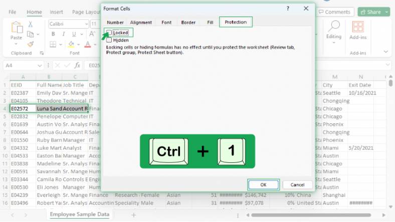
Shortcut 1. Lock a Cell

To lock a cell, select the cell and press Ctrl + 1 to open the Format Cells dialog box. Then, go to the Protection tab and check the “Locked” box. Click OK to save the changes. You can also right-click on the cell, select “Format Cells,” and follow the same steps.
2. Shortcut Unlock a Cell
To unlock a cell, select the cell and press Ctrl + 1 to open the Format Cells dialog box. Then, go to the Protection tab and uncheck the “Locked” box. Click OK to save the changes. You can also right-click on the cell, select “Format Cells,” and follow the same steps.
3. Shortcut Lock All Cells
To lock all cells in a worksheet, press Ctrl + A to select all cells. Then, press Ctrl + 1 to open the Format Cells dialog box. Go to the Protection tab and check the “Locked” box. Click OK to save the changes.
4. Shortcut Unlock All Cells
To unlock all cells in a worksheet, press Ctrl + A to select all cells. Then, press Ctrl + 1 to open the Format Cells dialog box. Go to the Protection tab and uncheck the “Locked” box. Click OK to save the changes.
5. Shortcut Lock a Range of Cells
Select the cells you want to lock to lock a range of cells. Then, press Ctrl + 1 to open the Format Cells dialog box. Go to the Protection tab and check the “Locked” box. Click OK to save the changes.
6. Shortcut Unlock a Range of Cells
Select the cells you want to unlock to unlock a range of cells. Then, press Ctrl + 1 to open the Format Cells dialog box. Go to the Protection tab and uncheck the “Locked” box. Click OK to save the changes.
7. Shortcut Lock a Row
To lock a row, select the row you want to lock. Then, press Ctrl + 1 to open the Format Cells dialog box. Go to the Protection tab and check the “Locked” box. Click OK to save the changes.
8. Shortcut Unlock a Row
To unlock a row, select the row you want to unlock. Then, press Ctrl + 1 to open the Format Cells dialog box. Go to the Protection tab and uncheck the “Locked” box. Click OK to save the changes.
You can also refer to these helpful articles on how to use Excel shortcuts:
9. Shortcut Lock a Column
To lock a column, select the column you want to lock. Then, press Ctrl + 1 to open the Format Cells dialog box. Go to the Protection tab and check the “Locked” box. Click OK to save the changes.
10. Shortcut Unlock a Column
To unlock a column, select the column you want to unlock. Then, press Ctrl + 1 to open the Format Cells dialog box. Go to the Protection tab and uncheck the “Locked” box. Click OK to save the changes.
FAQs
What is the primary purpose of locking cells in Excel?
Locking cells in Excel prevents accidental changes or edits to important data within a spreadsheet.
How can you quickly select an entire row in Excel using a keyboard shortcut?
Press Shift + Spacebar to select the entire row in Excel.
What is the purpose of protecting a worksheet in Excel?
Protecting a worksheet in Excel ensures that only authorized users can make changes to the structure and content of the spreadsheet.
How can you protect a workbook in Excel with a password?
Go to the “Review” tab, click on “Protect Workbook,” and choose “Protect with a Password.”
What is the purpose of protecting a workbook structure in Excel?
Protecting a workbook structure in Excel prevents users from adding, deleting, moving, hiding, or renaming worksheets within the workbook.
More in Excel

