


How to Freeze the Top Row and First Column in Excel
Microsoft Excel simplifies data management, and learning how to freeze the top row and first column is essential for efficient spreadsheet navigation. This guide provides clear instructions to help you quickly master this feature, improving data visibility and enhancing your overall Excel experience.

How to Freeze the Top Row and First Column in Excel
-
1. Freezing the Top Row in Excel
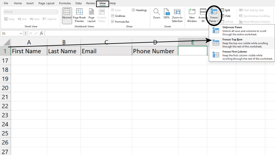
In Microsoft Excel, freezing the top row can significantly enhance your data analysis experience, especially when your top row serves as a header for the columns below. This feature allows you to scroll through your spreadsheet while keeping these crucial headers visible. To achieve this, first launch your Excel spreadsheet. Navigate to the ‘View’ tab, conveniently located on the ribbon at the top of your screen. Within the ‘Window’ section, you’ll find the ‘Freeze Panes’ option. Clicking on this reveals a dropdown menu, where you should select ‘Freeze Top Row.’ This action will lock the top row in place, allowing you to scroll down through your data.
-
2. Freezing the First Column in Excel
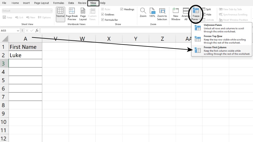
Similarly, freezing the first column in Excel is beneficial when it contains key identifiers for the rows. This function keeps these identifiers in sight as you scroll horizontally across your data. The process mirrors that of freezing the top row. Open your Excel file and head to the ‘View’ tab on the ribbon. Locate the ‘Freeze Panes’ feature in the ‘Window’ group and click it. From the options presented, choose ‘Freeze First Column.’ This action will anchor your first column, enhancing your ability to navigate large datasets.
-
3. Freezing Both the Top Row and First Column
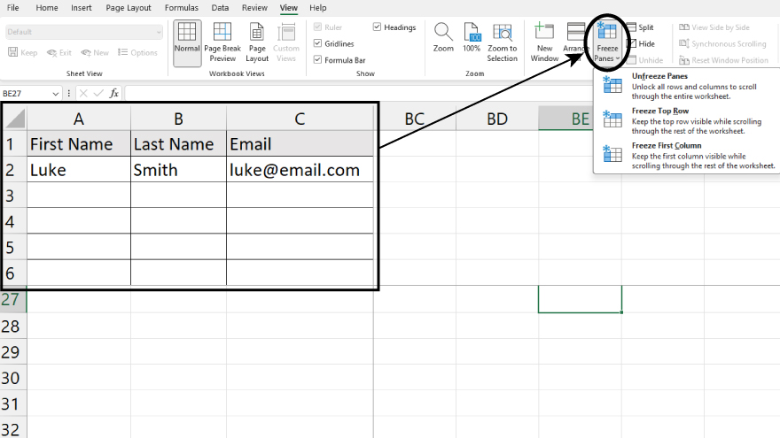
There are instances where you might need to freeze both the top row and the first column in Excel, especially when both contain essential labels or identifiers. To do this, open your spreadsheet and select cell B2. This step is crucial as Excel freezes rows and columns based on the cell’s position—it will freeze everything above and to the left of B2. After selecting the cell, go to the ‘View’ tab, and under the ‘Window’ group, click on ‘Freeze Panes.’ In the dropdown menu that appears, select ‘Freeze Panes.’ This will lock both the top row and the first column, facilitating a more comprehensive view of your data.
You can also refer to these helpful articles on how to use Excel shortcuts:
4. Unfreezing Panes in Excel
Unfreezing panes in Excel is a straightforward process that helps when you no longer need to keep specific rows or columns visible or when you wish to freeze a different section. To unfreeze, open your Excel document and access the ‘View’ tab. In the ‘Window’ group, click on ‘Freeze Panes.’ Within the dropdown menu that appears, select ‘Unfreeze Panes.’ This action will release any previously frozen rows or columns, allowing you to adjust your viewing preferences as your data analysis needs to evolve.
FAQs
How do I freeze the top row in Excel?
Select the ‘View’ tab, click ‘Freeze Panes,’ and choose ‘Freeze Top Row.’
Can I freeze both the top row and the first column simultaneously?
Yes, select cell B2, then click ‘Freeze Panes’ under the ‘View’ tab and select ‘Freeze Panes.’
How do I freeze the first column in Excel?
Go to the ‘View’ tab, click ‘Freeze Panes,’ and select ‘Freeze First Column.’
What happens when I freeze panes in Excel?
Freezing panes keeps selected rows or columns visible as you scroll through the spreadsheet.
How can I unfreeze panes in Excel?
Click ‘Freeze Panes’ under the ‘View’ tab and choose ‘Unfreeze Panes’ to revert the changes.
More in Excel

