


How to Unhide Column A in Microsoft Excel
Microsoft Excel provides an efficient solution for managing and presenting data, but sometimes essential columns like Column A can become hidden. Learning how to unhide Column A is crucial for accessing complete spreadsheet information and maintaining the integrity of your data.

How to Unhide Column A in Microsoft Excel
-
1. Using the Format Menu
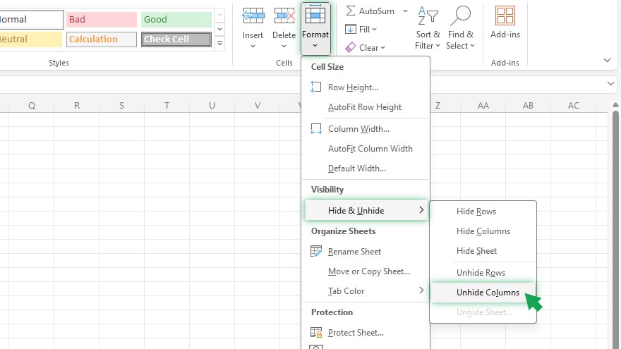
Accessing hidden columns in Excel can be effortlessly achieved through the Format menu. This user-friendly approach is ideal for beginners or occasional users. Start by selecting Column B’s header. Then, navigate to the Home tab, locate the Cells group, and click on ‘Format.’ Choose ‘Hide & Unhide’ from the dropdown list and select ‘Unhide Columns.’ This action will reveal Column A, ensuring complete visibility of your data. -
2. Employing the Go-To Dialog Box
The Go-To dialog box is an effective tool for handling large spreadsheets. Activate it by pressing F5, which opens a dialog box where you should enter ‘A1’ in the Reference field and click ‘OK.’ This action takes you to Cell A1 in the hidden Column A. Right-click on Column B’s header and select ‘Unhide’ from the context menu to reveal Column A.
-
3. Navigating with the Name Box
The Name Box, positioned next to Excel’s formula bar, is a versatile feature for navigating cells. To unhide Column A using this method, type ‘A1’ into the Name Box and press Enter. This brings you to Cell A1 in the hidden column. Right-click on the header of Column B and choose ‘Unhide’ from the context menu to make Column A visible.
You may also find valuable insights in the following articles offering tips for Microsoft Excel:
4. Applying Keyboard Shortcuts
For proficient Excel users, keyboard shortcuts offer a swift solution. To unhide Column A, the shortcut Ctrl + Shift + 0 (zero) can be used. Note that this shortcut might require activation in the Excel Options dialog box or may not be available in all Excel versions. For more tips about shortcut keys, check out the complete guide to Excel keyboard shortcuts.
5. Revealing Multiple Hidden Columns
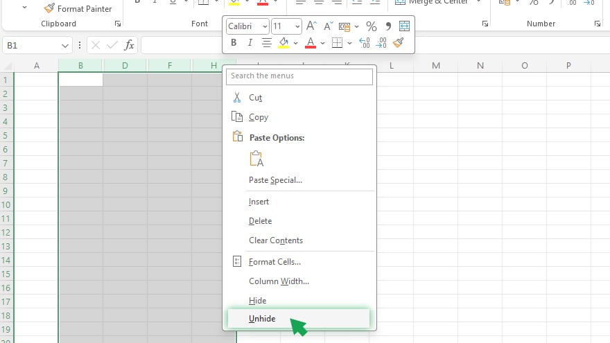
If your spreadsheet has several hidden columns, you can unhide them simultaneously. Click on the first visible column header to the right of the hidden columns, hold down Shift, and click on the last visible column header to the left of the hidden columns. Right-click on any of the highlighted headers and choose ‘Unhide’ from the context menu to reveal all hidden columns.
6. Preventing Column Hiding
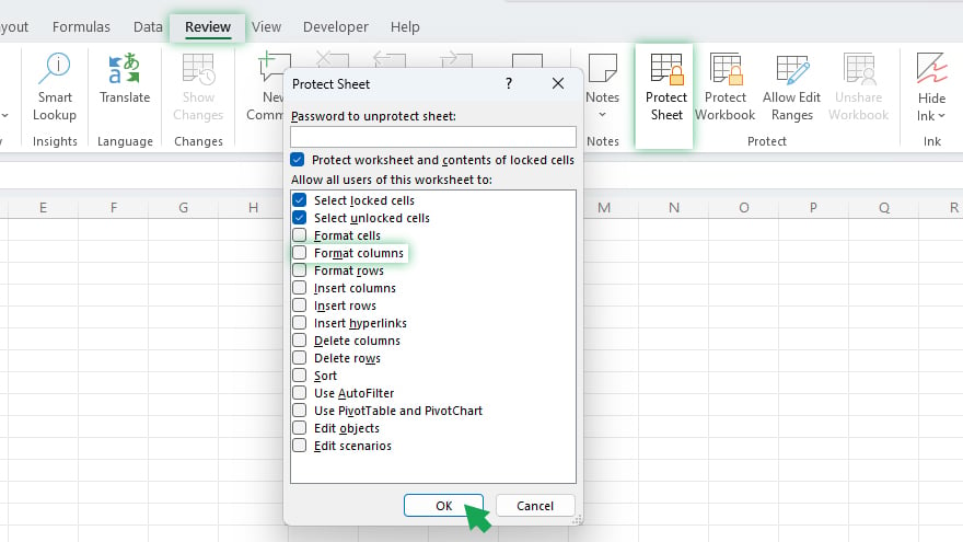
To safeguard your spreadsheet from unintentional column hiding, protect your worksheet. This can be done by going to the Review tab, selecting ‘Protect Sheet,’ and unchecking the ‘Format columns’ option. This prevents hiding columns while allowing other formatting changes.
FAQs
How do I unhide Column A using the Excel menu?
Select Column B, go to the Home tab, click ‘Format’ in the Cells group, and choose ‘Unhide Columns’ under ‘Hide & Unhide.’
Can I use a keyboard shortcut to unhide Column A in Excel?
Yes, press Ctrl + Shift + 0 (zero), but ensure this shortcut is enabled in your Excel settings.
Is it possible to unhide Column A using the Go-To dialog box?
Yes, press F5, type ‘A1’ in the dialog box, and right-click on Column B’s header to select ‘Unhide.’
How do I prevent columns from being hidden in Excel?
Protect the worksheet by going to the Review tab, clicking ‘Protect Sheet,’ and deselecting ‘Format columns.’
Can I unhide multiple columns, including Column A, at once?
Yes, select the headers of adjacent visible columns, right-click, and choose ‘Unhide’ from the context menu.
More in Excel

