


5+ How to Make an Inventory Using Excel – Tutorial
Microsoft Excel is one of the most adaptable professional tools in use today. Most of us already use it with its basic functions of tables and charts. One of the most important and most used functions of Excel is inventory management. Inventory management through Excel makes it easy to organize inventory while saving monetary and time values. MS Excel is more preferable for small and medium sized businesses where inventory counts to fewer items. In small businesses, Excel is an excellent option to manage inventory and keep records of sales and purchases, ordering and delivering and data keeping.

Excel offers various different simple inventory formulas to help in maintaining daily or routine business activities. To get the maximum out of it, the user should first know the need of using. Next comes the basic information about the business and entries to be made in inventory worksheet; i.e. What stock is at hand, what is demanded and what is to be delivered etc.
Inventory Spreadsheet Template in Excel

Inventory Checklist Template in MS Excel

Inventory Sign Out Sheet Template

Small Business Legal Compliance Inventory Template

Sample Inventory Control Template

Simple Inventory Template

Home Inventory Sheet Template

Small Business Inventory Template

Stock Inventory Control Template

Create Your Own Inventory
Excel provides an updated record of all business activities and also provides the relaxation from looking into loads of paperwork. Now let’s have a look in to step-by-step process of creating inventory using MS Excel.
Step 1
Launch Microsoft Excel. A blank spreadsheet ready for the inventory form opens. 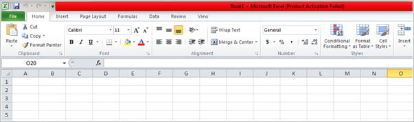
Step 2
Click into cell A1, the first on the spreadsheet. Type “S. No.”, “Product ID”,“Product Number”,“Catalog Number”, or your preferred way of tracking inventory items. For a simple basic inventory we will start with Product ID. 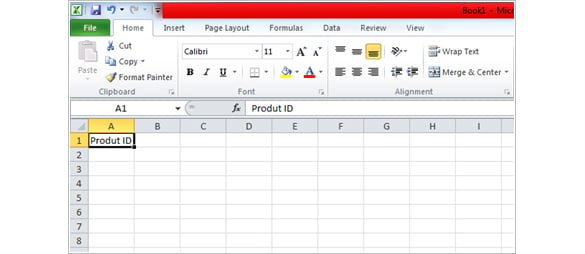
Step 3
Click on cell B1 or press the “Tab” key on keyboard to move next cell on the right i.e. B1. Type “Receiving”, “In Date”, “Inventory In” or your preferred term to track when you have received an item. 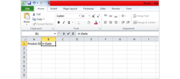
Step 4
In the similar manner, enter header entries “Shipped”, “Initials”, “Out Date” and “Comments” in the cells C1, D1, E1 and F1 respectively. This will make the headers of inventory complete. Now you have basic heads under which your inventory will be created. 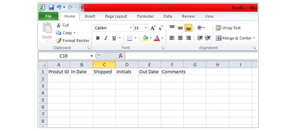
Step 5
Place the cursor on columns on the line between columns A and B and click twice. This will adjust the column width of column A to adjust the content of the cell. Repeat the same for all the columns. For the Comments column, place the cursor on the line between columns F and G, click and hold to increase column to your desirable width. 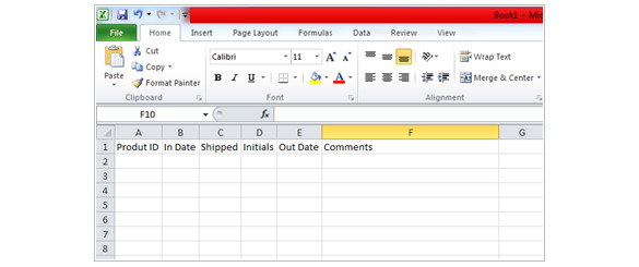
Step 6
Now it’s time for some formatting and giving the inventory a professional and presentable look. First of all, you need a title for the inventory. Place the cursor on row 1 and click to highlight the complete row. Right click on “1” and select “insert”. This will insert a blank row above the Headers. Type the name of inventory here. 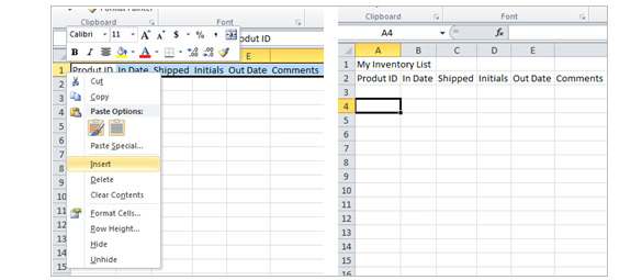
Step 7
Highlight the title, increase the font size to18. Place the cursor on cell A1 and drag it across to F1. Then click “Merge & Center” button in the Alignment group on Home tab. You can also give a shade to the title through fill color option in the Font group. 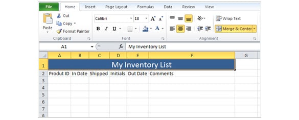
Step 8
The header should be more prominent than the listed items. For this highlight all the header columns. Increase the font size to 14, options for which are available in Font group in the Home tab. Click on “B” to give boldface to the headers. Next you can give the header and distinguished color and also further highlight them by add color to header cells through Fill Color option. All these formatting options are available in the Font group in Home tab. 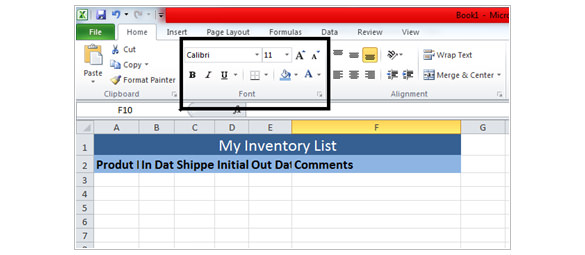
Step 9
As you can see, the cells and columns are over lapping. This can be easily adjusted by adjusting the width of columns. Repeat Step 5 to fix the issue of column width. 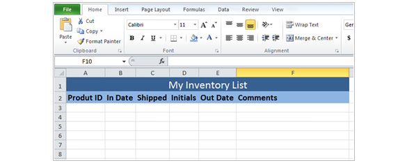
Step 10
Add border to the inventory to give it a cleaner look. Let’s suppose, your inventory has 10 items; select the cell A1 and then drag it down to A12 and across to F12. Now, select ‘All Borders’ from drop-down border list. Then select the My Inventory List and select ‘Thick Box Border’ from the same list. Your inventory list should look much more professional and neat. 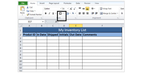
Step 11
Select row 3. Go to “View” tab and then click “Freeze Panes.” Select “Freeze Panes” from the drop-down menu. Now you will never miss sight of your header, no matter how many inventories you will add or how far you go down the spreadsheet. 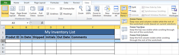
Step 11
Now you inventory worksheet is ready to be worked. Before start working on it, it is highly recommended to save the file. Go to file tab and click “Save As.” Enter a name of your choice, such as “My Inventory List”. Click the “Save” button.
Use a Template
MS Excel also has its own preset templates for inventory management. The user can pick an inventory template from his choice from this list as well. These are pre-made templates with complete formatting and formulae inserted. These can be often very handy. Let’s see how we can use them.
Step 1
Open Excel 2010, click “File” taband then click “New.” 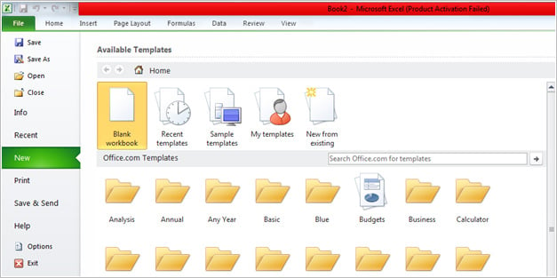
Step 2
Select “Inventories” from the list of template types that appear. A list of inventory template options will display. 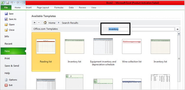
Step 3
Browse through the list of inventory templates. While browsing, you can see a live preview on the side bar of the window. Select the one that is suitable for your business and purpose. 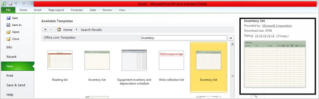
Step 4
Click “Download” to open the selected template. 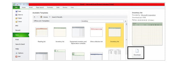
Step 5
The template comes with formatting already done; however, it is customizable and you can make any alterations to the inventory as you wished to in order to make it more professional and appealing and relevant to your business.
Step 6
Save the spreadsheet with a filename of your choice.
Conclusion
Excel can be an extremely useful tool for small businesses, especially if you know how to make use of it to its best effect. One the best benefit of Excel is it reduces the manual labor and traumatic data entry.
More in Tutorials

